Coefficient | Model 1 |
|---|---|
(Intercept) | 1.26 |
aid_pct | 0.10 |
democracy | 0.23 |
aid_pct | 0.50 ** |
N | 40 |
R sq. | 0.5 |
Adj. R sq. | 0.46 |
Significance: ***p < .01; **p < .05; *p < .1 | |
Seminar on Interaction Effects with R
An example with easytable
Alfredo Hernandez Sanchez
Vilnius University
2026-04-30
When should we use interaction terms?
When the effect of a predictor variable \(x_1\) on the response variable \(\widehat{y}\) is not independent from another predictor \(x_2\)
For example, the interaction term tells us whether the relationship between \(x_{1}\) and \(\widehat{y}\) is different when \(x_{2} = 1\) compared with when \(x_{2} = 0\).
Multivariate OLS
\[ \widehat{y} = \beta_{0} + \beta_{1}x_{1} + \beta_{2}x_{2} + \epsilon \]
Where
- \(\widehat{y}\) is the dependent variable
- \(\beta_{0}\) is the intercept
- \(x_{1}\) is an independent variable
- \(x_{2}\) is another independent variable
- \(\epsilon\) is the error term
Regression with interaction term
\[ \widehat{y} = \beta_{0} + \beta_{1}x_{1} + \beta_{2}x_{2} + \beta_{3}(x_{1} \times x_{2}) + \epsilon \]
Where:
- \(\beta_{3}\) is the coefficient for the interaction between \(x_{1}\) and \(x_{2}\)
- the effect of \(x_{1}\) on \(\widehat{y}\) depends on the value of \(x_{2}\)
Interpreting the interaction terms
Assume \(x_{1}\) is continuous and \(x_{2}\) is binary.
When \(x_{2} = 0\):
\[ \widehat{y} = \beta_{0} + \beta_{1}x_{1} \]
When \(x_{2} = 1\):
\[ \widehat{y} = (\beta_{0} + \beta_{2}) + (\beta_{1} + \beta_{3})x_{1} \]
\(\beta_{2}\) is the change in the intercept when \(x_{2} = 1\).
\(\beta_{3}\) is the change in the slope of \(x_{1}\) when \(x_{2} = 1\).
Binary Interaction Results
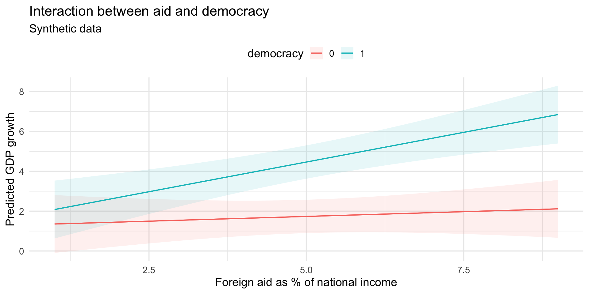
Example of an interaction
Suppose we want to study whether foreign aid is associated with economic growth (RQ). But we suspect that aid does not work the same way everywhere.
- H: Aid may be more useful when the state has stronger administrative capacity.
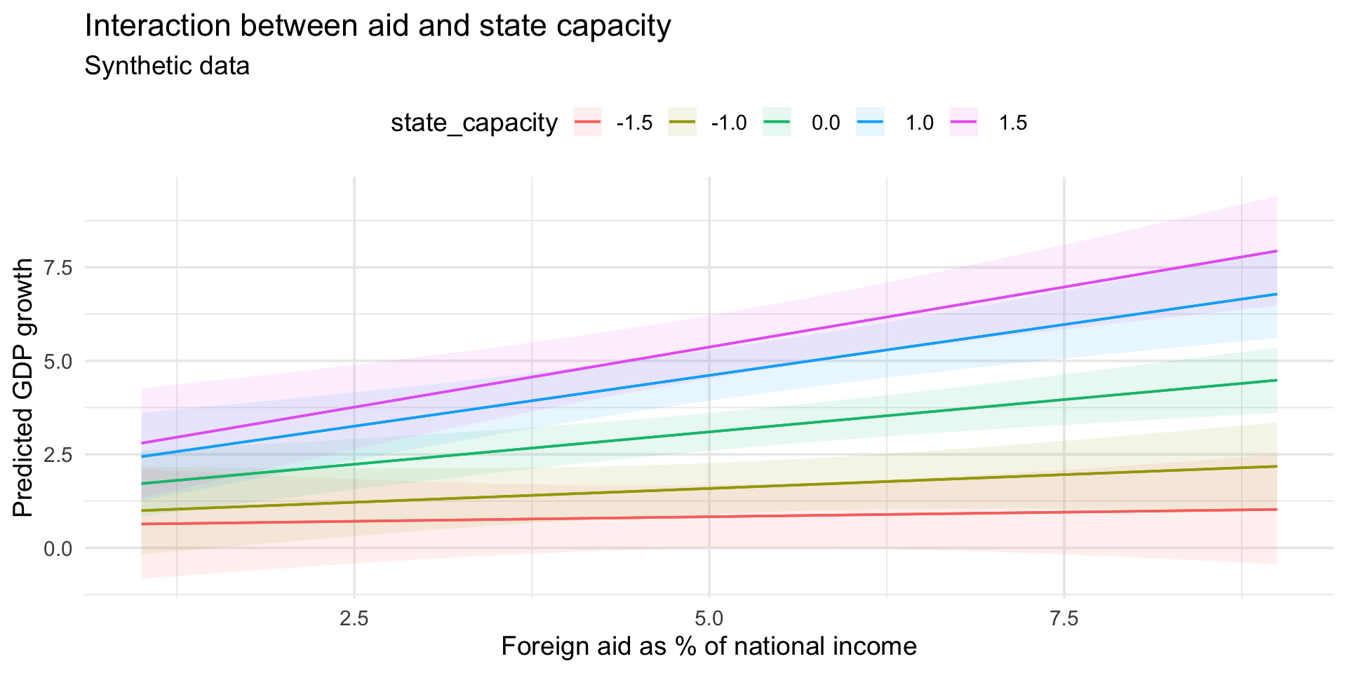
\[ \widehat{Growth} = 1.37 + 0.35 Aid + 0.52 Capacity + 0.20(Aid \times Capacity) \]
Where
- \(Growth\) is annual GDP growth
- \(Aid\) is foreign aid as a percentage of national income
- \(Capacity\) is a state capacity index (median centered)
- \(Aid \times Capacity\) is the interaction term
Interpretation
The effect of aid is not just \(0.35\).
Because aid is interacted with state capacity, the effect of aid is:
\[ \frac{\partial \widehat{Growth}}{\partial Aid} = 0.35 + 0.20 Capacity \]
For every one-point increase in state capacity, the association between aid and predicted GDP growth becomes 0.2 percentage points stronger.
Results
Coefficient | Model 1 |
|---|---|
(Intercept) | 1.37 ** |
aid_pct | 0.35 *** |
state_capacity | 0.52 |
aid_pct | 0.20 ** |
N | 40 |
R sq. | 0.64 |
Adj. R sq. | 0.61 |
Significance: ***p < .01; **p < .05; *p < .1 | |
Interaction Terms in R
Coefficient | Model 1 | Model 2 | Model 3 |
|---|---|---|---|
(Intercept) | 1.37 ** | 1.37 ** | 1.35 *** |
aid_pct | 0.35 *** | 0.35 *** | 0.10 *** |
state_capacity | 1.51 *** | 0.52 | 0.53 *** |
aid_pct | 0.20 ** | 0.20 *** | |
democracy | 0.24 * | ||
population_m | -2.14E-3 | ||
aid_pct | 0.50 *** | ||
N | 40 | 40 | 40 |
R sq. | 0.58 | 0.64 | 0.99 |
Adj. R sq. | 0.55 | 0.61 | 0.99 |
Significance: ***p < .01; **p < .05; *p < .1 | |||
Reporting regression results with easytable
Install easytable
easytable() vs summary()
Call:
lm(formula = gdp_growth ~ aid_pct + state_capacity, data = df)

Residuals:
   Min     1Q Median     3Q    Max
-3.515 -1.321  0.022  1.369  3.330

Coefficients:
               Estimate Std. Error t value Pr(>|t|)
(Intercept)     1.37244    0.55819   2.459  0.01874 *
aid_pct         0.34556    0.09717   3.556  0.00105 **
state_capacity  1.51190    0.24582   6.150 3.93e-07 ***
---
Signif. codes:  0 '***' 0.001 '**' 0.01 '*' 0.05 '.' 0.1 ' ' 1

Residual standard error: 1.738 on 37 degrees of freedom
Multiple R-squared:  0.577, Adjusted R-squared:  0.5542
F-statistic: 25.24 on 2 and 37 DF, p-value: 1.221e-07Comparing models with easytable()
Coefficient | Model 1 | Model 2 |
|---|---|---|
(Intercept) | 1.37 ** | 1.37 ** |
aid_pct | 0.35 *** | 0.35 *** |
state_capacity | 1.51 *** | 0.52 |
aid_pct | 0.20 ** | |
N | 40 | 40 |
R sq. | 0.58 | 0.64 |
Adj. R sq. | 0.55 | 0.61 |
Significance: ***p < .01; **p < .05; *p < .1 | ||
Other easytable() commands
Coefficient | Model 1 | Model 2 | Model 3 |
|---|---|---|---|
(Intercept) | 1.37 ** | 1.37 ** | 1.35 *** |
aid_pct | 0.35 *** | 0.35 *** | 0.10 *** |
state_capacity | 1.51 *** | 0.52 | 0.53 *** |
aid_pct | 0.20 ** | 0.20 *** | |
democracy | 0.24 * | ||
population_m | -2.14E-3 | ||
aid_pct | 0.50 *** | ||
N | 40 | 40 | 40 |
R sq. | 0.58 | 0.64 | 0.99 |
Adj. R sq. | 0.55 | 0.61 | 0.99 |
Significance: ***p < .01; **p < .05; *p < .1 | |||
# Name models, set digits
easytable(m1, m2,
          digits = 1,
          model.names = c("A", "B"),
          highlight = TRUE)
Coefficient | A | B |
|---|---|---|
(Intercept) | 1.4 ** | 1.4 ** |
aid_pct | 0.3 *** | 0.3 *** |
state_capacity | 1.5 *** | 0.5 |
aid_pct | 0.2 ** | |
N | 40 | 40 |
R sq. | 0.58 | 0.64 |
Adj. R sq. | 0.55 | 0.61 |
Significance: ***p < .01; **p < .05; *p < .1 | ||
Export and set control variables
Coefficient | Model 1 | Model 2 | Model 3 |
|---|---|---|---|
(Intercept) | 1.37 ** | 1.37 ** | 1.35 *** |
aid_pct | 0.35 *** | 0.35 *** | 0.10 *** |
state_capacity | 1.51 *** | 0.52 | 0.53 *** |
aid_pct | 0.20 ** | 0.20 *** | |
democracy | 0.24 * | ||
aid_pct | 0.50 *** | ||
population_m | Y | ||
N | 40 | 40 | 40 |
R sq. | 0.58 | 0.64 | 0.99 |
Adj. R sq. | 0.55 | 0.61 | 0.99 |
Significance: ***p < .01; **p < .05; *p < .1 | |||
Summary
library(easytable)
mtcars

# Define models
m1 <- lm(mpg ~ wt, data = mtcars)
m2 <- lm(mpg ~ wt + hp, data = mtcars)
m3 <- lm(mpg ~ wt + hp + cyl + am, data = mtcars)

# Table
easytable(m1, m2, m3,
          control.var = c("cyl", "am"),
          model.names = c("A", "B", "C"),
          export.word = "table.docx",
          export.csv = "table.csv",
          highlight = TRUE)
Activity
Work in pairs or groups of 3.
Your task is to use the gapminder data to test one interaction effect.
- Choose an outcome variable, such as
lifeExp - Choose one main explanatory variable, such as
log_gdp - Choose a second variable that may change the relationship, such as
continent,pop, or a dummy variable (binary) you create - Write one simple hypothesis
- Write one short mechanism explaining why the interaction might exist
- Estimate a regression model with an interaction term
- Interpret the interaction coefficient in plain English
Thank you for your attention!
About the FIRSA Project
Disclaimer:
This project has received funding from the European Union Marie Skłodowska-Curie Postdoctoral Fellowships / ERA Fellowships action under grant agreement No. 101180601 under the title: Understanding FinTech Regulatory Sandbox Development in Europe (FIRSA).
Learn more at the project website.

This project has received funding from the European Union Marie Skłodowska-Curie Postdoctoral Fellowships / ERA Fellowships action under grant agreement No. 101180601 under the title: Understanding FinTech Regulatory Sandbox Development in Europe (FIRSA).
Learn more at the project website.
![]()